Neural Architecture Search (NAS)- The Future of Deep Learning

Most of us have probably heard about the success of ResNet, winner of ILSVRC 2015 in image classification, detection, and localization and Winner of MS COCO 2015 detection, and segmentation. It is an enormous architecture with skip connections all over. While using this ResNet as a pre-trained network for my machine learning project, I thought “ How can someone come out with such an architecture? ’’

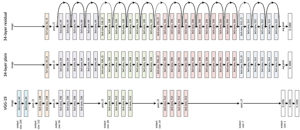Large Human Engineered Architecture

Soon after I learned that many engineers and scientists with their years of experience build this architecture. And there is more of a hunch than complete math that will tell you “ we need to have a 5x5 filter now to achieve the best accuracy ’’. We have wonderful architectures for the image classification task, but for other tasks, we have to spend much of our energy to find an architecture with reasonable performance for those tasks. It would certainly be better if we can automate this architecture modeling task just as we learn the parameters of machine learning models.

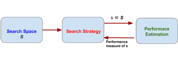
Neural Architecture Search (NAS), the process of automating architecture engineering i.e. finding the design of our machine learning model. Where we need to provide a NAS system with a dataset and a task (classification, regression, etc), and it will give us the architecture. And this architecture will perform best among all other architecture for that given task when trained by the dataset provided. NAS can be seen as a subfield of AutoML and has a significant overlap with hyperparameter optimization. To understand NAS we need to look deeply into what it is doing. It finds an architecture from all possible architectures by following a search strategy that will maximize the performance. The following figure summarizes the NAS algorithm.

Dimensions of NAS method

It has 3 separate dimensions: Search Space, Search Strategy, and Performace Estimation.

Search space defines what neural architecture a NAS approach might discover in principle. It can be chain-like architecture where the output of layer (n-1) is fed as an input of layer (n). Or it can be a modern complex architecture with skip connection (multi-branch network).

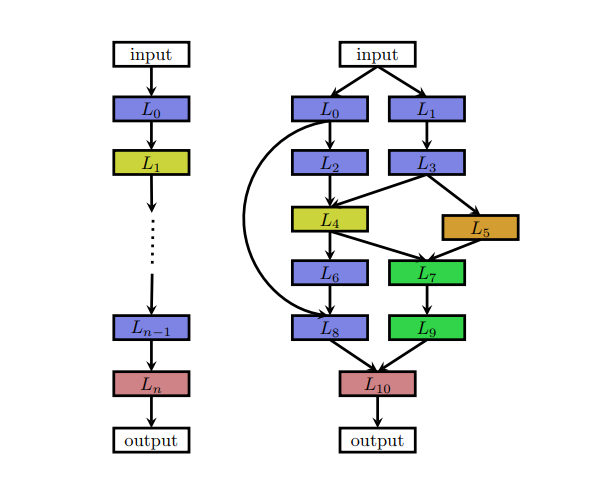A chain-like and multi-branch network

Sometimes people do want to use handcrafted outer architecture( macro-architectures) with repeated motifs or cells. In such cases, the outer structure is fixed and NAS only searches for the cell architectures. This type of search is known as micro-search or cell search.

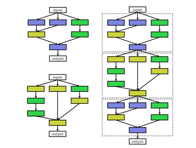left: The cell architecture right: cells are put in the handcrafted outer structure

In many NAS methods, both micro and macro structures are searched in a hierarchical fashion; which consists of several levels of motifs. The first level consists of the set of primitive operations, the second level of different motifs that connect primitive operations via a directed acyclic graph, the third level of motifs that encode how to connect second-level motifs, and so on.

To explain the search strategy and performance estimation, three different NAS methods will be discussed in the following part.

Reinforcement Learning

Reinforcement learning is the problem faced by an agent (a program) that must learn behavior through trial and error interactions with a dynamic environment to maximize some reward. An agent( performs some action according to some policy parametrized by θ. Then that agent updates the policy θ from the reward for that action taken. In the case of NAS, the agent produces the model architecture, child network( the action). Then the model is trained on the dataset and the performance of the model on the validation data is taken as a reward.

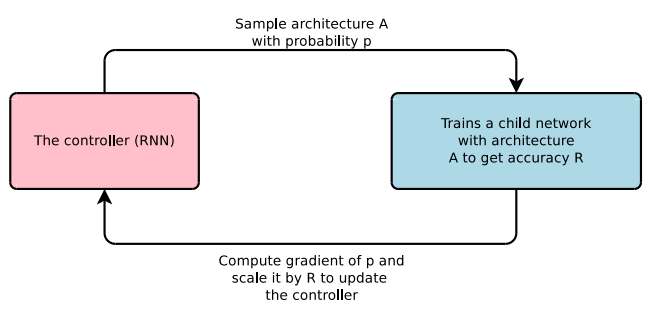The controller plays the role of an agent and accuracy is taken as the reward

In general, a Recurrent Neural Network (RNN) is taken as a controller or agent. It produces string and the model is built form that string stochastically.

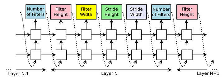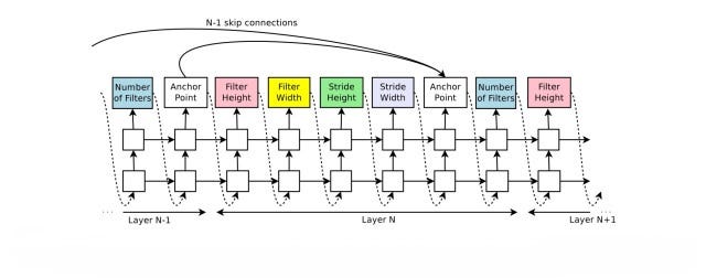
RNN predicts filter height, filter width, stride height, stride width, and the number of filters for one layer and repeats in a form of string. Each prediction is carried out by a softmax classifier and then fed into the next time step as input. The RNN stops after generating a certain number of outputs.

A sample output for such RNN is shown in the above figure. The hyperparameters for each layer of a convolutional neural net are produced repeatedly up to a certain number of times. And then a model is then built following the output of RNN, which is then trained and validation accuracy is calculated.

Here, the parameters of RNN acts as the policy θ of the agent. Production string (height, filter width, stride height, etc) is the action of the agent. The performance of the model on the validation set is the reward of the agent in this reinforcement method. The RNN updates its parameters θ in a way such that, the expected validation accuracy of the proposed architectures is maximized.

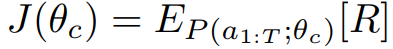
The RNN is trained by a policy gradient method to iteratively update the policy θ. The main target is to maximize the expected accuracy i.e.

Here R is the accuracy of the model, a1: T is the string of length T produced by RNN( the action), θ is the parameter of RNN.

As J(θ) is not differentiable, a policy gradient method is used to iteratively update θ. The update function looks like

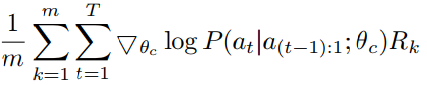
This is an approximation of the original equation. The expectation term of J(θ) is replaced by sampling. The outer summation of this updated equation is for that sampling i.e. m numbers of models sampled from RNN and their average is taken. P(a_t|a_(t−1):1; θc), is the probability of taking an action a_t at time t given all actions from 1 to (t-1) according to policy θ or predicted by RNN with parameter θ.

Example of strings produced by RNN to create a model

Encoding skip connections is a bit tricky. For this RNN for each layer generates an output called the Anchor point. The anchor point is used to indicate skip connections. At layer N, the anchor point will contain N − 1 content-based sigmoids to indicate the previous layers that need to be connected.

Progressive Neural Architecture Search (PNAS)

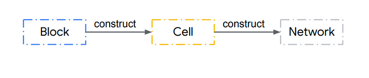
PNAS does a cell search as discussed in the search space part of this tutorial. They construct cells from blocks and construct the Complete network by adding the cells in a predefined manner.

Hierarchy of model architecture

Cells are connected in a series in a predefined number to form the network. And each cell is formed by several blocks( 5 used in the original paper).

Add caption

The blocks consist of predefined operations.

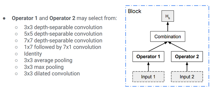structure of a block. The Combination function is just an element-wise addition

Operations that have shown in the figure are used in the original paper and can be extended.

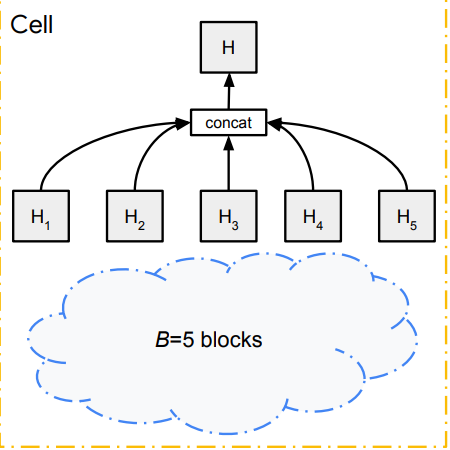
the complete structure of a Cell

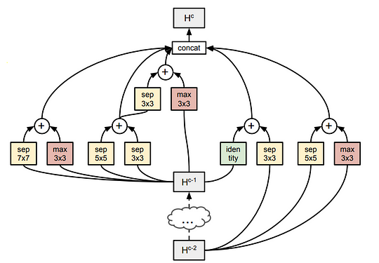
On the left, an example of a complete is shown. Even in this cell or micro search, there are in total 10 ¹⁴ valid combinations to check to find the best cell structure.

So, to reduce complexity first only cells with only 1 block are constructed. It is easy because with the mentioned operation there are only 256 of different cells that are possible. Then top K best-performing cells are chosen to expand for 2 block cells and it is repeated up to 5 blocks.

But for a reasonable K, too many 2-block candidates to train. As a solution to this problem, a “cheap” surrogate model that predicts the final performance simply by reading the string(cell is encoded into a string) is trained. The data for this training is collected when the cells are constructed, trained, and validated.

For example, we can construct all 256 of single block cells and measure their performance. And train the surrogate model with this data. Then use this model to predict the performance of 2 block cells without training or testing them. And of course, the surrogate model should be capable of handling variable size input. And then top K best performing 2 block cells as predicted by the model is chosen. These 2 block cells are then trained, the “surrogate’’ model is finetuned and these cells are expanded to 3 blocks and it is iterated until we get 5 block cells.

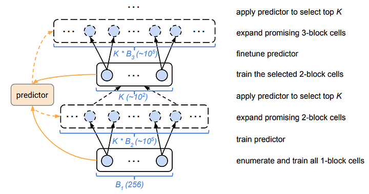Steps in PNAS

Differentiable Architecture Search (DARTS)

The search space for neural architectures is discrete i.e one architecture is different from the other by at least a layer or some parameter in the layer, for example, 5x5 filter vs 7x7 filter. In this method, continuous relaxation is applied to this discrete search which enables direct gradient-based optimization.

The cell we search can be though as a directed acyclic graph where each node x is a latent representation (e.g. a feature map in convolutional networks) and each directed edge (i, j) is associated with some operation o(i,j) (convolution, max-pooling, etc) that transforms x(i) and stored a latent representation at node x(j)

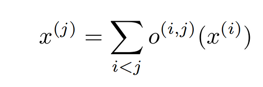
the output of each node can be calculated by the equation on the left. The nodes are enumerated in such a way, that there is an edge(i,j) from node x(i) to x(j), then i<j.

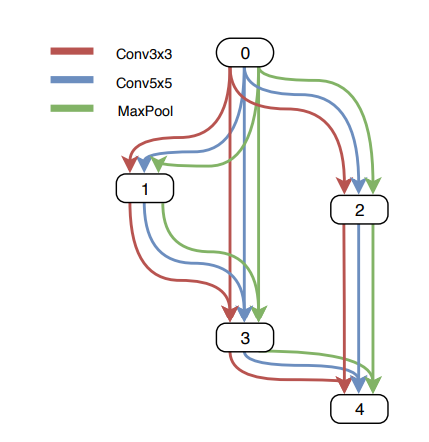
In continuous relaxation, instead of having a single operation between two nodes. a convex combination of each possible operation is used. To model this in the graph, multiple edges between two nodes are kept, each corresponding to a particular operation. And each edge also has a weight α.

continuous relaxation of the discrete problem

Now O(i,j) the operation between node x(i) and x(j) is a convex combination of a set of operations o(i,j) where o(.)ϵ S, where S is the set of all possible operations.

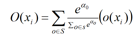
The output of O(i,j) is calculated by the left equation.

The training and the validation loss are denoted by L_train and L_val respectively. Both losses are determined not only by the architecture parameters α but also by the weights ‘w’ in the network. The goal for architecture search is to find α∗ that minimizes the validation loss L_val(w ∗ , α∗ ), where the weights ‘w∗’ associated with the architecture is obtained by minimizing the training loss.

w∗ = argmin L_train(w, α∗ ).

This implies a bilevel optimization problem with α as the upper-level variable and w as the lower-level variable:

α * = argmin L_val(w ∗ (α), α)

s.t. w ∗ (α) = argmin L_train(w, α)

After training some α’s of some edges become much larger than the others. To derive the discrete architecture for this continuous model, in between two nodes the only edge with maximum weight is kept.

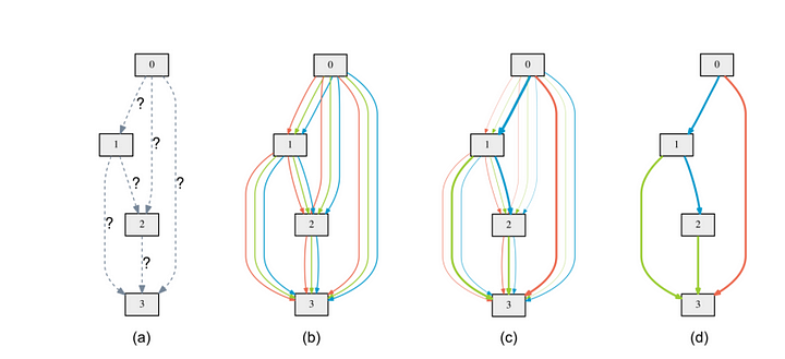a) Operations on the edges are initially unknown. b) Continuous relaxation of the search space by placing a mixture of candidate operations on each edge c) some weights increases and some falls during bilevel optimization d) final architecture is constructed only by taking edges with the maximum weight between two nodes.

When the cells are found, these are then used to construct larger networks.

There are many other methods that are also used in neural architecture search. And they achieved an impressive performance. But still, we have very little knowledge for answering the question ‘why does a particular architecture work better?’. I think we are on our way to answering that question.

References

1. Deep Residual Learning for Image Recognition
2. Neural Architecture Search: A Survey
3. NEURAL ARCHITECTURE SEARCH WITH REINFORCEMENT LEARNING
4. Progressive Neural Architecture Search
5. DARTS: DIFFERENTIABLE ARCHITECTURE SEARCH