Human beings along with many other animals have 5 basic senses: Sight, Hearing, Taste, Smell, and Touch. We also have additional senses like a sense of balance and acceleration, a sense of time, etc. Every single moment the human brain processes information from all these sources and each of these senses affects our decision-making process. During any conversation, movement of lips, facial expression along with sound produced by vocal cord helps us to fully understand the meaning of words pronounced by the speaker. We can even understand words only by seeing the lips movement without any sound. This visual information is not just supplementary but necessary. This was first exemplified in the McGurk effect (McGurk & MacDonald, 1976) where a visual /ga/ with a voiced /ba/ is perceived as /da/ by most subjects. As we want our machine learning models to achieve human-level performance, it is also necessary to enable them to use data from various sources.
In machine learning these type of data that comes from different heterogeneous sources are known as multimodal data. For example audio and visual information for speech recognition. It is difficult to directly use these multimodal data in the training, as they may be of different dimensionality and data types. So much of the attention is paid to learning a common representation of these multimodal data. Learning common representations for such multiple views of data will help in several downstream applications. For example, learning a common representation for videos and their audios could help in generating more accurate subtitles for that video than if it generated by only using audio. But how do you learn this common representation?
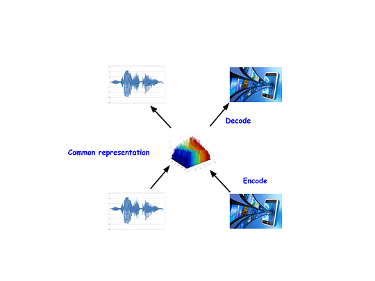 |
| An abstract view of CorrNet. It tires to learn a common representation of both views of data and tries to reconstruct both the view from that encoded representation. |
Correlational neural network (CorrNet) is one of the methods for learning common representations. Its architecture is almost the same as a conventional single-view deep autoencoder. But it contains one encoder-decoder pair for each modality of data.
Let’s consider a two-view input, Z = [Ia, Iv], where Ia and Iv are two different views of data such as audio and video. In the figure below, one simple architecture of CorrNet with this data is shown.
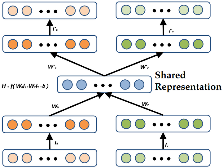 |
| Example of CorrNet with bimodal data Z = [Ia, Iv] where Ia and Iv are two different views of data like (audio and video )Add caption |
Where both encoder and decoder are single-layered. H is the encoded representation. Ha = f( Wa.Ia+b) is encoded representation Ia. f() is any non linearity ( sigmoid, tanh , etc.). Same is the case of Hv = f( Wa.Ia+b). And the common representation of bimodal data Z is given as :
H = f(Wa.Ia + Wv.Iv + b).
In the decoder part, the model tries to reconstruct the input from the common representation H by I’a = g(W’a.H+b’) and I’v = g(W’vH+b’), where g() is any activation and I’a and I’v is the reconstructed Inputs.
During training, the gradient is calculated based on three losses:
i) Minimize the self-reconstruction error, that is, minimize the error in reconstructing Ia from Ia and Iv from Iv.
ii) Minimize the cross-reconstruction error, that is, minimize the error in reconstructing Ia from Iv and Iv from Ia.
iii) Maximize the correlation between the hidden representations of both views, that is, maximize the correlation between Ha and Hv.
The total loss can be written as
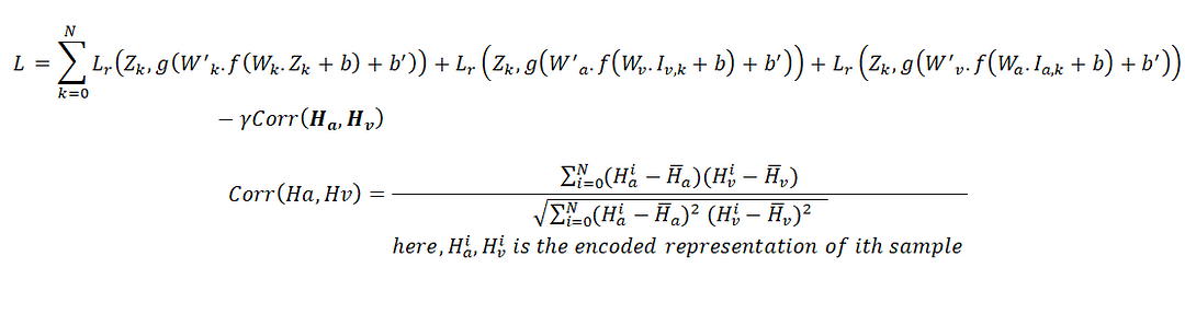
Here, Lr() represents reconstruction loss which may be ‘mean squared error’ or ‘mean absolute error’. Our target is to minimize this loss. And as we want to increase the correlation, it is subtracted from the loss, i.e., the higher is the correlation the lower is the loss.
Implementation
Total implementation can be divided into three parts: Model Building, Setting loss functions, and Training.In the Model Building phase, we have to create that auto encodes architecture. First, we have to include all the necessary packages| from keras import Model |
| from keras.layers import Input,Dense,concatenate,Addfrom keras import backend as K,activationsfrom tensorflow |
| import Tensor as Tfrom keras.engine.topology |
| import Layer |
| import numpy as np |
| #Then we have to create CorrNet architecture. For simplicity, it has a single-layered encoder and decoder. |
| class ZeroPadding(Layer): |
| def __init__(self, **kwargs): |
| super(ZeroPadding, self).__init__(**kwargs) |
| def call(self, x, mask=None): |
| return K.zeros_like(x) |
| def get_output_shape_for(self, input_shape): |
| return input_shape |
| #inputDimx,inputDimy are the dimentions two input modalities. And #hdim_deep is the dimentions of shared representation( kept as #global veriable) |
| hdim_deep = 10 #dimenstion of shared representation |
| inpx = Input(shape=(inputDimx,)) |
| inpy = Input(shape=(inputDimx,)) |
| #Encoder |
| hl = Dense(hdim_deep,activation='relu')(inpx) hr = Dense(hdim_deep,activation='relu')(inpy) h = Add()([hl,hr]) #Common representation/Encoded representation |
| #decoder |
| recx = Dense(inputDimx,activation='relu')(h) recy = Dense(inputDimy,activation='relu')(h) |
| CorrNet = Model( [inpx,inpy],[recx,recy,h]) |
| CorrNet.summary() |
| '''we have to create a separate model for training this CorrNet. During training, we have to take a gradient from 3 different loss |
| functions and which can not be obtained from a single input. If you look closely at the loss function, we will see it |
| has different input parameters.''' |
| [recx0,recy0,h1] = CorrNet( [inpx, inpy]) |
| H= concatenate([h1,h2]) |
| model = Model( [inpx,inpy],[recx0,recx1,recx2,recy0,recy1,recy2,H]) |
| [recx1,recy1,h1] = CorrNet( [inpx, ZeroPadding()(inpy)])[recx2,recy2,h2] = CorrNet( [ZeroPadding()(inpx), inpy ]) |
| #Now we have to write the correlational loss function for our model. |
| Lambda = 0.01 |
| #by convention error function need to have two argument, but in #correlation loss we do not need any argument. Loss is computed #competely based on correlation of two hidden representation. For #this a 'fake' argument is used. |
| def correlationLoss(fake,H): |
| y1 = H[:,:hdim_deep] |
| y2 = H[:,hdim_deep:] |
| y1_mean = K.mean(y1, axis=0) |
| y1_centered = y1 - y1_mean |
| y2_mean = K.mean(y2, axis=0) |
| y2_centered = y2 - y2_mean |
| corr_nr = K.sum(y1_centered * y2_centered, axis=0) |
| corr_dr1 = K.sqrt(K.sum(y1_centered * y1_centered, axis=0) + 1e-8) |
| corr_dr2 = K.sqrt(K.sum(y2_centered * y2_centered, axis=0) + 1e-8) |
| corr_dr = corr_dr1 * corr_dr2 |
| corr = corr_nr / corr_dr |
| return K.sum(corr) * Lambda |
| def square_loss(y_true, y_pred): |
| error = ls.mean_squared_error(y_true,y_pred) |
| return error |
| #Now we have to compile the model and train |
| model.compile(loss=[square_loss,square_loss,square_loss, square_loss,square_loss,square_loss,correlationLoss],optimizer="adam") |
| model.summary() |
| '''Suppose you have already prepared your data and kept one moadlity data in Ia(e.g. Audio) and another in Iv( e.g. Video). |
| To be used by this model Audios and videos must be converted into 1D tensor.''' |
| model.fit([Ia,Iv],[Ia,Ia,Ia,Iv,Iv,Iv,np.ones((Ia.shape[0],Ia.shape[1]))],nb_epoch=100) |
| np.ones((Ia.shape[0],Ia.shape[1])) is fake tensor that will be passed to correlationLoss function but will have no use |
| '''using this model we can generate Ia to Iv.For example, from video Iv we can generate corresponding audio Ia |
| np.zeros(Ia.shape) gives tensors of 0 of dimestions same as output tensor audio.''' |
| audio,_,_ = CorrNet.predict([np.zeros(Ia.shape),Iv]) |
After training, the common representation learned by this model can be used in different prediction tasks. For example, common representations learned using CorrNet can be used for: cross-language document classification or transliteration equivalence detection. Various studies have found that using common representation increases performance. It can also be used in data generation. For example, in a certain dataset, you have 10000 audio clips with corresponding videos, 5000 audio clips with their videos missing, and 5000 videos with their audios missing. In such cases, we can train a CorrNet with 10000 audios and videos and can be used to generate missing videos for audio and vice versa.